NEWFIRM Detectors
Detector Characterization
Based upon a report provided by M. Bonati (30 August 2023)
1. Introduction
- Characterization of the four NEWFIRM arrays was carried out while the instrument was installed in the Blanco Cass cage. Illumination was provided by the dome flat (white spot) lights.
- All of the images were taken using the JX filter.
- The full characterization was done using 400 mV biasing. Some tests were repeated using 600 mV and 800 mV biasing.
- All of the light tests were done using spatial measurements only (no temporal measurements). The noise tests were done using both spatial and temporal measurements.
- In all the graphs, the detector order is: (UL) SCA022, (UR) SCA011, (LL) SCA023, and (LR) SCA019
1.1 Evaluated parameters
- Low-light variance (Gain)
- High-light variance (linearity, gain versus mean well)
- Noise versus number of samples
- Dark current
- Inter pixel capacitance (IPC) / hot pixels
- Image persistance
- Well / Dark / IPC / Noise versus detector biasing
2. Summary of results
(average of all four arrays)
| Item | Result | Unit |
| Noise1 | 45 | e- |
| Noise4 | 22.5 | e- |
| Gainlow | 7.5 | e- ADU-1 |
| Gainhigh | 9.9 | e- ADU-1 |
| Well | 100 | Ke- |
| NL100Ke | <2 | % |
| Dark30k | 0.18 | e- pix-1sec-1 |
| IPC | 2.9 | % |
| Hot pixels | 0.0014 | % |
| Persistence tc | 12 | sec |
3. Low-light variance
Counts up to 3000 ADUs only to examine the behavior under relatively low light conditions. A series of two images per illumination level were taken. Using one image per level, we derived the linearity curve, shown in Figure 1.

Figure 1: Linear fit of exposure times versus counts for each of the arrays, under low light conditions.
Using each pair of images, we determined the gain using the variance curve technique. The fit results can be see in Figure 2. The gain values derived for each detector can be seen in Table 2.

Figure 2: Linear fit of each of the array variances under low light conditions.
Table 2: Low Illumination Results
| Detector | Gain (e- ADU-1) | NL (%) |
| SCA022 | 8.1 | 0.2 |
| SCA013 | 7.2 | 0.3 |
| SCA011 | 7.1 | 0.2 |
| SCA019 | 7.4 | 0.4 |
4. High-light variance
Going up to saturation, this test examines the behavior of the arrays under relatively high-intensity light conditions. From this test, we also derive the full well of each array, based on the maximum non-linearity (NL) desired. A series of two images per illumination level were taken. Using one image per level we also determined the linearity curve, shown in Figure 3. The NLL residual averages and individual full wells are also shown in Figure 3. The point at which the NL exceeds 2% is considered to be the full well.


Figure 3: (Top) Linear fit of each array. (Middle) Average residuals and the actual value of each array in ADUs for NL < 2%. This represents the full well. (Bottom) Individual NL residuals for the linear fits.
Using each pair of images, only up to the point where they meet the desired NL, we derived the gain using the variance curve technique. The fit can be seen in Figure 4 (top). However, because NIR devices are intrinsically non-linear, the gain is also a function of illumination level. By calculating the 2nd derivative of the variance curve, we obtain a "gain versus mean" curve that can be seen in Figure 4 (bottom). The red dots are an attempt to an exponential fit, but in reality it is a more accurate approach to assume a fixed gain of around 7.5 to 8 if the mean value is below 6000 ADU and either use a linear fit after that or simply leave it fixed around a value ~9-10. The actual gain values determined from the the linear fit to each array can be found in Table 3. In the same table, we added the full well for each detector in electrons, calculated by multiplying the gain and the maximum value in ADUs before reaching saturation. The last column shows the NL up to that full well value.


Figure 4: (Top) Linear fits to each array's variance curves. (Bottom) Gain versus mean function.
Table 3: High Illumination Results
| Detector | Gain (e- ADU-1) | Full well (ke-) | NL (%) |
| SCA022 | 10.1 | 119 | 1.7 |
| SCA013 | 9.9 | 115 | 1.1 |
| SCA011 | 9.8 | 110 | 1.1 |
| SCA019 | 9.8 | 99 | 0.9 |
5. Noise
The noise was calculated by taking fifteen images for each sample value (Fowler sampling), of 1, 2, 4, and 16. For each sample the images were normalized and then noise was calculated in three separate ways:
- Spatial: Using a standard deviation of a selected spatial area for each of the images, then average the standard deviations.
- Image Histograms: Making a histogram of all of the images for each sample, the fitting a Gaussian and calculating the mode of the histogram, then averaging the mode value.
- Full histogram: Combining all fifteen images, then fit a Gaussian to determine the mode of the combined images.
Figure 5 shows all of the results in the same plot. They coincide reasonably well, all of them indicating a clear deviation from the theoretical value, in this case because the images were not time-corrected. Figure 6 shows the Gaussian fits for the full histograms. Table 4 shows the final results, using the full histogram modes multiplied by the average gain under low light conditions (see Table 2).

Figure 5: All methods are shown above. The spatial, amp histogram (image histogram, and full histogram.

Figure 6: Accumulated (full) histograms for each Fowler sampling value.
Table 4: Noise Scan
| Fowler | Full Histogram Noise (e-) |
| 1 | 41.2 |
| 2 | 30 |
| 4 | 23 |
| 16 | 12.5 |
6. Darks
To calculate the dark current, we took a sequence of ten images per exposure time, from 0 sec to 360 sec in steps of 45 sec. Each set of images was median-filtered to obtain one master dark per exposure time. We then calculated the dark current in three different ways:
- Using the mode of each master image (Gaussian fit), we made a curve of exposure time versus mode and fit a line. The slope provides the vale of the dark current. This is shown in Figure 7 (top).
- We took the highest exposure master file, normalized by the minimum, divided by the differential exposure time and multiplied by the gain to obtain a dark fits image. We then calculated the dark current of each array (mode of each extension) as shown in Figure 7 (middle) and Table 4.
- We took the dark fits image from the previous step and calculated the mode of the histogram with all extensions combined as shown in Figure 7 (bottom)


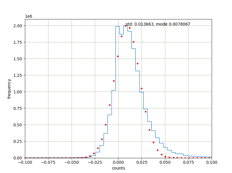
Table 4: Dark Current per Array (e- pix-1sec-1)
| Array | Dark Current |
| SCA022 | 0.12 |
| SCA011 | 0.08 |
| SCA013 | < 0.1 |
| SCA019 | 0.21 |
Table 5 shows a summary of the three different methods and Figure 8 shows the master dark image.
Table 5: Average Dark Current (e- pix-1sec-1)
| Slope | Combined Histogram | Average Arrays (e- pix-1sec-1) |
| 0.16 | 0.06 | 0.1 |

7: Inter Pixel Capacitance (IPC) and hot pixels
We used the dark current images to calculate the inter pixel capacitance (IPC). We located the isolated "hot pixels" that had values greater than 5000 over the background. For each hot pixel we determined the value of all of the pixels surrounding it (using s 3 x 3 matrix) and then subtracted the overall background. Next, we added the charge on all nine pixels and normalized them as a percent of the total charge. We did the same for all hot pixels, obtaining a mean and standard deviation value for each pixel position. The result can be seen in the top panel of Figure 9. To verify that the dependence of the IPC versus the the signal value, we plotted the hot pixel values against its calculated IPC. As can be seen in the figure, the trend is to keep a similar percentage, regardless of the the signal value (Figure 9 center panel). A summary of the IPC value per surrounding pixel is shown in Table 6 as well as the total (addition of charge for all pixels). The value obtained is well inside the expected range, usually less than 6%. With the isolated hot pixels, we generated a hot pixel map per array as shown in the bottom panel of Figure 9. The hot pixels correspond to 0.0014% of all pixels.
Table 6: IPC per pixel matrix (%)
| 0.116 ± 0.09 | 0.519 ± 0.27 | 0.11 ± 0.08 |
| 0.68 ± 0.35 | 96.6 ± 1.14 | 0.75 ± 0.32 |
| 0.13 ± 0.09 | 0.48 ± 0.27 | 0.12 ± 0.10 |


![]()
Figure 9: (Top) IPC per surrounding pixel. (Middle) IPC percentage as a function of hot pixel value. (Bottom) Hot pixel map of the arrays.
8: Biasing variations
We computed the most important parameters against other array biasing. The results for full well, darkk current, IPC, and noise can be found in Table 7 below. The behavior is as expected: full well increases with biasing, but dark current and IPC increase considerably. The noise seems unaffected excepted for the floor in the 800 mV case where it also increases considerably (see Figure 10).
Table 7: Parameter variation as a function of array biasinng
| Parameter | 400 mV | 600 mV | 800 mv |
| Full well | 10500 | 11170 | 12420 |
| Dark e- | 0.18 | 0.27 | 1.28 |
| IPC | 2.9 | 3.5 | 7.0 |
| Noise16 | 1.7 | 1.9 | 2.1 |
 |
 |
 |
 |
Figure 10: Parameter variations as against detector biasing.
9: Image persistence
In order to measure persistence the arrays were flushed with a quartz lamp mounted in the Blanco chimney. Unfortunately, we were unable to generate a well-focused spot. We did however, get saturated areas on one of the arrays (SCA013) that allowed us to measure persistence (see Figure 11). We exposed the FPA until it reached 8000 ADUs (i.e., maximum linear range), then took a long series of minimum exposure images.After some hours, we repeated the test until 10000 ADUs were reached (i.e., saturation), and again until 16000 ADUs (i.e., deep saturation) were reached.
We computed the mean on the saturated region for each of the cases (see Figure 11) and then measured the mean in the same region in subsequent dark exposure images. We then performed an exponential fit to these data. The results can be seen in the bottom panel of Figure 11. Surprisingly, the level of saturation does not seem to matter as in other NIR devices and the persistence corresponds in all cases to a simple exponential with a time constant of approximately 12 seconds. This implies that the array is free of long-delivery traps and only has rapid-release ones. Effectively, after integrating on a very bright object, the effect of image persistence will be reduced by 95% in approximately one minute. We assume this holds true for the other NEWFIRM arrays but it needs to be properly measured.


Figure 11: (Top) Image persistence from saturated light and the subsequent dark images. (Bottom) Model of perstitence for linear, saturation, and deep-saturation regions.
Updated on May 29, 2025, 12:19 pm