The DECam Community Pipeline Instrumental Signature Removal


The DECam Community Pipeline
Instrumental Signature RemovalFrancisco Valdes, August 2021
frank.valdes@noirlab.eduTable of Contents
1. Introduction
The Dark Energy Camera [DECam, 2015] is a workhorse instrument on the Victor M. Blanco 4m Telescope at the Cerro Tololo Inter-American Observatory (CTIO) -- a division of NSF's National Optical-Infrared Research Laboratory (NOIRLab). In support of this instrument the NOIRLab Community Science and Data Center (CSDC) operates a science pipeline, called the DECam Community Pipeline or DCP, to provide instrumentally calibrated, science quality data products to observing programs and, ultimately, a community archive of DECam data. This paper describes the calibration methods where "calibration" means the removal of instrumental signatures.
The DCP, like all pipelines, has a life history running from a rapidly evolving initial state to a slower evolving, mature state. A static state only occurs at the end of life which is not currently the case. Therefore, a description of the pipeline is for a particular version. This document is for version 5, though many aspects are the same for earlier versions.
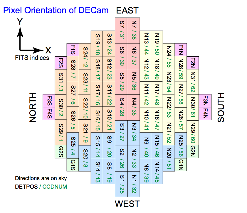
DECam consists of 62 2kx4k CCDs (with 12 ancillary guiding and focus detectors) each read out with 2 amplifiers (see figure 1) [DECam CCDs]. Of these one CCD has been unusable (N30/61) and one has had an unstable amplifier (S7/31) for most of DECam's operation. Another CCD (S30/02) ceased imaging for several years but produces useable data from both before and after this period. Therefore, the instrumental calibration is for 60 or 61 CCD images but with one CCD not recommended for science use.
The DCP functionality, calibrations, corrections, and products are presented in the following sections. §2 briefly describes the workflow and requirements for the raw data, though that is not the principle topic of this document. It also introduces the point that while there is a standard default calibration workflow and data products, there can be variations depending on programs and user needs. §3 is a quick description of image segmentation which is a key algorithmic step in several of the calibration operations. §4 describes the creation of master dome calibrators that precede science processing. The core instrumental function of the DCP, namely flux calibration, is described in §5. The astrometric calibration, which provides a mapping of pixel to celestial coordinates through a world coordinate system (WCS) function, follows in §6. Determining a characteristic magnitude zero point is in §7. Flux calibration doesn't necessarily produce a uniform background so §8 describes handling of the background from the sky and stray light. §9 presents projecting the exposures to a standard, undistorted, pixel sampling. The projected exposures are stacked (aka coadded), with a number of options, as described in §10. There are various sources of unusable or scientifically suspect pixels which are identified and flagged as described in §11. The last §12, describes the final data products. Depending on the nees and desires of the programs not all data products may be produced. The order of these sections do not represent the orchestration order of the pipeline workflow where many of the steps are intertwined.
Figure 1: DECam Focal Plane and CCD Identifiers [DECam CCDs]
2. Orchestration and User Requests
Orchestration is about what data is processed and how the workflow is executed by the pipeline infrastructure. While this is not the focus of this document there are some aspects of this that can impact the programs, are relavant to the to the following sections, and can be subject to user needs. Normally data orchestration and the calibration options are at the discretion of the pipeline scientist and operator based on an understanding of the program described in the proposal abstract and the efficient operation of the pipeline.
The DCP processes "datasets" which are any collection of raw exposures. The operator normally choses datasets by program, night, or run. But other datasets can be defined as needed or requested. The operator also sets processing options based on the type of program and the observer or requester's needs. Requests for special datasets is the most common form of user interaction with the DCP.
There are a variety of calibration and algorithmic options in the DCP. A default processing usually occurs shortly after the data is taken. A common question is "when are the DCP data products available?". It is not possible to provide a specific timescale for various reasons including the overall data volume for programs and possible hardware problems (which can lead to a backlog). In general, the operator attempts to complete a program within days or a week of the end of a run. Data may also be available the day after an observing run for many programs; especially those with near-real time needs.
In addition to requesting expedited processing, observers or archival users may request non-default options. In the sections that follow many of the alternatives are indicated. It is always useful to discuss program requirements and desires with the DCP operators.
Datasets are divided into exposures to be ignored (i.e. bad), zero bias sequences, dome flat sequences, and science exposures. The dome sequences are grouped by night. The dome flat and science exposures are also divided by filter and processed independently and often in parallel.
"Bad" data consists of exposures externally labeled as bad, those corrupted in some way (which generally are recovered if the corruption happened during data transport), missing or invalid required keywords, and those whose titles indicate they are or tests of various types. Note that the word "test" itself does not cause exclusion. Observers can flag exposures to skipped by the DCP by including the case insensitive word "junk". Table 1 summarizes the causes for exposures to be skipped by the DCP.
Observers can communicate bad exposures to be skipped by the DCP. But since the pipeline normally will produce data products even from bad data without impacting operations, this is usually left for the users of the data products to exclude later. If titles ignored by the DCP are desired the form of titles needs to be communicated to the operator.
Another important type of bad data are any exposures with the CCD voltages turned off or turned on in the preceding exposure since the first exposure after the camera is activated are unusable. Typically, activation occurs before dome calibrations and ignoring the first calibration exposure is part of the routine. However, cycling the camra could occur during the night.
Table 1: Causes for Excluded Exposures
Ignore In bad list, first exposure after turning on detector voltages, dark, sky flat Keywords
(Missing/invalid)EXPTIME, OBSTYPE, MJD-OBS, FILTER, PROPID, SATURAT?, TELRA, TELDEC Title words
(case insensitve)Junk, pointing, focus, donut, AOS, AMap, PPMap Table 2: Orchestraion Options
Details Operation Default Description §2 Dataset list Operator The operator normally selects exposures from a night or run. Users may request special datasets by supplying a list of exposures (numbers or archive names). A remote triggering option, usually during observing, is possible with advance arrangements. CCDs to process All This is used by the operator when CCDs (single or a controller group) are unusable. This could be used for special user needs; particularly for quicker turnaround. Exclude from stacks 31 CCDs to exclude in stacks. Partially bad CCDs in dithered stacks can imprint throughout much of the stack. This is normally an operator option to deal with the unstable amplifer in DECam without totally excluding it from other data products.
3. Image Segmentation
A fundamental capability in pipelines and science analysis is segmenting images into sources and background. Most commonly, segmenting images is used for creating catalogs. But in pipelines the ability to create masks for the sources and separate out the sky is also very important. Because this type of operation occurs multiple times in the DCP we provide some details in this section to avoid repeating them later.
The DCP makes use of two segmenting tools. Because of historical legacy the widely known Source-Extractor [SExtractor 1996] program produces the source catalogs used for astrometric solutions (§6) and photometric characterization (§7). the lesser known IRAF Astronomical Cataloging Environment [ACE 2001] is used for source characterization, masking, background sky determination and flattening, and image difference transient detection. This package was designed around producing the various types of segmentation products useful in pipeline algorithms: catalogs, object masks, two types of sky images, sky variance images, and image difference segmentation. It was also designed so the products work seamlessly with other IRAF tools; especially the object masks. This is clearly appropriate since most of the DCPs functionality comes from IRAF tools and script modules.
The purpose of the SExtractor catalogs is clear including as the natural input to the astrometry solver SCAMP [SCAMP 2006]. The ACE catalogs are used to parametrically identify cosmic rays and satellite trails. They are also used in image difference mode as part of moving object detection when there are multiple exposures. The source masks are used for defining removal of bad data by interpolation, in algorithms for background template fitting (pupil and fringe), and when unregistered stack are produced for dark sky illumination. The binned and unbinned sky images are used for pupil
It is the sky background function that requires further description. The sky is determined in 64x64 pixel blocks. A histogram is made of unmasked pixels and the mode determined. An iterated standard deviation around the mode is computed and the sky value is the mean in a 3 standard deviation window about the mode in the histogram. When a sky value can't be determined in a block the sky value is filled in by interpolation from nearby blocks. The block values can be output as a binned "mini-sky" image. The sky values and sigma values can also be output at the size of the image by interpolation.
4. Master Dome Calibrators
As is typical of CCD cameras, DECam observing includes taking sequences of exposures for zero bias and flat field calibration. The exposures are routinely taken by observing support staff. Zero bias exposures are taken with the shutter closed (and with blocking filters) and a commanded exposure time of zero. Flat field exposures are taken of an illuminated "white" screen in a darkened dome. To minimize noise contributions from these calibrators, sequences of consecutive exposures with optimal exposure times are taken.
The nightly dome calibration sequences are processed first and in the order of zero bias and dome flats. The sequences are processed into coadded master calibrations. For random reprocessing the dataset lists don't contain dome calibration exposures and the appropriate master calibrations are expected to have been created and available in the DCP calibration library. The order of bias, dome flat, and science processing allows the result of the preceding step to be applied to the data in the next step.
The initial instrumental calibration steps are performed on all exposures -- dome calibrations and science alike. These operations are header updates (thus far just resetting saturation levels), crosstalk corrections, saturated pixel identification, electronic (overscan) bias subtraction, and masking of light from "hot" pixels . Apart from the zero bias exposures, they are also corrected for non-linearity. These operations are described in subsequent sections.
Zero bias sequences for each night are stacked into a master zero bias. The pixels at each point in the mosaic array are averaged with the highest and lowest values excluded. The inverse variance, referred to henceforth as weights, of each pixel are estimated from the pixel statistics and engineering values for readout noise and gain measurements and stored as a weight map. The master zero files are available from the archive.
The dome flat sequences for each filter are corrected for bias by a master zero bias, scaled by their medians, and stacked as the average with the high and low value excluded. The master bias applied is the chronologically nearest which is almost always from the same night. The median of the dome flat is computed in a central region with bad pixels excluded. The weights are estimated from the pixel statistcs and readout noise and gain values for the amp and include the uncertainties in the bias introduced by the bias subtraction. The weights are saved in a weight map for use in the science calibrations. The master dome flats are available in the archive.
Figure 2 displays typical bias and dome flats in the g, r, and z filters. Fine details are not visible due to the size of the field and the gain differences of the CCDs which dominate the flat fields.
Figure 2: Typical Bias and Dome Flat Master Calibrations from 2019-03-07.
The zero bias is displayed between -2 to 5 counts and the dome flats from +/- 20% about the global mean normalization. Upper-left is zero bias, upper-right is g-band, lower-left is r-band, and lower-right is z-band.
5. Flux Calibrations
The primary purpose of an instrumental pipeline is to transform the raw instrumental pixel counts to linear values with uniform proportionality with respect to flux from the sky. The first steps are to make the transformed values zero when there is no light and then make the proportionality with flux (known as the gain) be the same for all pixels at all signal levels. Pixels that can't be transformed to scientifically useful values are identified and recorded in a data quality mask as discussed in §11.
In summary, the flux calibrations are correction for nonlinearity, correction for electronic crosstalk, removal of electronic bias, application flat fields for gain uniformity and variable pixel sizes, and adjustments for electrostatic effects. Another correction sometimes applied is for CCD dark current. This is not done by the DCP as the dark current has a negligible effect on DECam exposures. The methods and details of these corrections and calibrations are provided in the rest of this section.
Estrada et al. (2010) reported DECam CCD nonlinearity at both low fluxes and near saturation as determined from flat field images. The DCP corrects for this nonlinearity with an amplifier-dependent lookup table that converts bias subtracted counts to linear counts (G. Bernstein et al. 2017, in preparation). The lookup table has not changed since initial commissioning. Figure 3.A shows the linearity behavior as the numerical derivative of the lookup table; i.e. departure from an ideal linear function. The curves for all the amplifiers are superimposed to illustrate the similarities and variation of the linearity. In an ideal linear detector the curves would be at one for all raw count values.
The camera, as is typical of parallel channel readout electronics, has some crosstalk. DECam has 70 CCDs, each with two amplifiers, read out in parallel. The crosstalk correction consists of scaling the signal from one amplifier and subtracting it from another amplifier. The scaling is defined by a set of coefficients (constant up to a level near saturation and then quadratic). Figure 3.B plots the coefficients as the excess crosstalk contribution to an affected pixel from a 50,000 count pixel in another amplifier; i.e. the crosstalk coefficient multipled by 50,000. There are three cases in the plot. The white symbols show the excess in amplilfier A when the source pixel is in amplifier B of the same CCD, the red symbols for the effect of amplifier B from amplifier A on the same CCD, and the green symbols for the effect on a CCD (in either amplifier) from a different CCD. In general crosstalk is strongest between amplifiers on the same CCD rather than between CCDs.
Figure 3: DECam Linearity and Crosstalk
The left figure shows linearity curves for all amplifiers superimposed as a function of raw counts. These are computed by numerical differentiation of the linearity look-up table.
The right figure shows the crosstalk coefficients represented as the excess crosstalk signal at 50,000 counts as a function of CCD number. The white symbols are for the effect on amplifier A by amplifier B on the same CCD, the red are for the effect on amplifier B by amplifier A on the same CCD, and the green are the effect on either amplifier by amplifiers in other CCDs.
The standard electronic bias corrections apply the overscan data taken at the end of each row readout and a average zero bias pattern. The ovrscan corrections accounts for bias variations at the time scale of individual line readouts while the zero bias correction is patterns that are static over times scales of a night. There are no suspected bias variations (often called pattern noise) on intermediate time scales.
The average overscan value, with the highest and lowest excluded, is subtracted from each row. While there are options for first fitting the overscan correction over all rows to reduce sampling noise, this is be strongly discouraged because the parallel readout of the focus and guiding CCDs, which have half the number of rows, introduces a jump in raw counts when they finish reading out. Any signal bias is corrected by subtraction of a master zero bias as described previously.
The static zero bias pattern, represented by the master zero bias images described in §4, is removed by subtraction.
Flat fielding is the process of correcting each pixel to the same gain assuming a linear behavior following the linearity correction. There are a number of commonly used techniques. The DCP includes these and applies then in an iterative order where each step is a correction to the the previous ones. It also provides for temporal changes in the corrections by deriving calibrations on various time scales.
The first, and most common method, is application of a dome flat field. This is a nightly master calibration image as described in §4. The DCP uses the nearest available in time for each exposure. This allows for possible variations in the camera gains and for potentially missing or compromised such as by warming of the camera. Note that this makes the response to the projected dome screen uniform and includes, as do all the flat field operations, measuring uniform counts even though the optical pixel sizes are not perfectly uniform. The normalized flat field calibrations image is applied by division and the statistical effects of the noise in the flat field and the science exposure are recorded in an inverse variance weight map.
The next technique is based on photometry of stars. This method is variously called photometric flats, star flats, or "thousand points of light". The same stars are dithered spatially such that the same stars appear on multiple amplifiers and CCDs. Then a response pattern that minimizes the photometric differences, after dome flat fielding, is generated. The method optimizes photometric uniformity for the typical colors of the stars rather than the dome projection or dark sky. But since it can only sample a subset of pixels it requires interpolation to define the response for every pixel. This type of flat field is also only generated a few times a year during observatory calibration time. The nearest photometric flat in time is applied to the exposures. The software used to produce the photometric flats from the calibration exposures is that of Bernstein [Bernstein 2017].
Ideally the dome flat field accounts for the difference in the gains of the two amplifiers from each CCD. Due to the limitations of converting the star photometry to a continuous photometric flat field that calibration does not provide for amplifier gain differences. In practice there are noticeable background level differences in some of the CCDs. Whether these are color differences between the dome and sky illumination is unclear. Because the algorithm described next is based on the median behavior over the dataset it is a kind of illumination correction.
The current default calibration workflow applies an amp gain balancing step. A median stack of all exposures for each CCD is created. The mean value of a 100 pixel strip on each side of the amplifier boundary is measured and a gain balance correction is computed to match the mean of the B amplifier to the A amplifer. To avoid gross errors limits are placed on the correction. First the correction is reduced by 20%. Then for CCDs 29 and 45 the maximum correction is set to zero; i.e. no correction. For CCD 31 a correction up to 100% is permitted. For the u and narrow band filters a maximum correction of 20% is allowed. For all other filters a maximum of 5% is placed. If the correction is greater than these bounds or if the correction is less than 0.05% then no correction is applied. It is the case that some CCDs have amp difference exceeding the maximum allowed correction so these are left unchanged.
The last common technique is dark sky illumination flat fields. This is based on producing uniform response to sky. These require datasets with a sufficient number of well dithered and measurable sky background exposures. As opposed to star flats this provides illumination of all pixels and can be generated more frequently from the program observeration but is different photometrically because the color of the sky is not the same as typical stars. It also suffers from the challenge that the sky is not really uniform due to other sources of additive light. When these are generated the operator inspects them to ensure no source light is being imprinted on the result.
The DCP generates dark sky illumination images by combining unregistered images with sources masked by ACE and with some statistical rejection. This is done after the sky uniformity corrections described in §8. The stack is then smoothed, since it is rare there is enough clear data at each pixel, by amplifier and with a variable smoothing scale to follow more rapid variations near the CCD edges. These flat fields are applied in the usual fashion by normalizing over all CCDs and dividing into the science exposures. Note that dark sky illumination images may be used instead as a sky flattening step rather than as a flux calibration step.
Dark sky illumination images, either for gain or sky uniformity, are options and are currently not used by default. It can be useful for narrow band programs.
An example grayscale rendering of the three types of flat field calibrations is shown in fig. 4. These are selected as the nearest available in time. For bias and dome the master calibrations are typically from the same night as the exposure. For the photflat these are only generated periodically. Illumation flats were generated from runs with many exposures. Use of illumination flats was deprecated when star flats became available at different epochs. The calibrations used are documented in the data product headers.
Figure 4: Dome Flat, Star Flat, and Illum Flat
These are r-band flat fields. (left) Dome flat +/- 20%, (middle) Star flat +- 20%, (right) Dark sky illumination flat +/- 1%.
Table 3: Flux Calibration Options
Details Operation Default Description CCD ops skip bf Standard CCD calibration to skip. The calibrations are static bad pixel flags, linearity, zero bias, dome flat, photometric flat, "brighter-fatter", and amp gain balancing. The default is all operations but the "brighter-fatter" correction. Dark sky flat skip Create and apply a dark sky illumination flat. 6. Astrometry
Astrometric calibration consists of matching stars in an exposure with an astrometric reference catalog and fitting a world coordinate system (WCS) function mapping image pixel coordinates to celestial coordinates for each CCD. The WCS function for a CCD is a 3rd order bidimensional polynomial distortion followed by tangent plane projection in a FITS formalism, called TPV [TPV 2011].
The source catalogs for each CCD are generated by SExtractor [SExtractor 1996]. These are matched against the 2MASS reference catalog (PLVER < 3.10), Gaia DR1 (PLVER between 3.11 and 4.1), and Gaia DR2 (PLVER > 5.0). The source catalogs include celestial coordinates evaluated from the instrumental pixel centroids, a predefined library WCS, and the pointing supplied at the telescope. The matching is done by SCAMP [SCAMP 2006]. A vaild match requires the matching statistics (number of stars, RMS, and Chi^2) to meet certain thresholds.
There are a number of reasons the matching may fail with the most common one being low transparency, i.e. clouds, producing few or no stars. During this and subsequent steps a failure results in a header keyword indicating the failure.
Each CCD has a predetermined WCS function that defines the CCD position and orientation in the mosaic array relative to a tangent point near the center of the field. It also includes a higher order distortion map. The predetermined distortion maps were derived by the DES project [DES Pipeline, 2018]. The same maps have bee used in all DCP processing.
These library WCS functions correct each star to a nominal undistorted astrometric coordinate. The astrometric solution then fits a 3rd order polynomial to adjust the tangent point, orientation, and a constrained large scale distortion across the mosaic array to minimize the errors in the match to the astrometric catalog. The solution is then exported to the CCD header WCS in the TPV formalism [TPV 2011]. This solution method essentially keeps the predetermined metrology with allowance for a constrained distortion of the focal plane. There are no proper motion or epoch adjustments currently.
7. Photometric Characterization
A photometric characterization provides a magnitude zero point (MAGZERO, MAGZPT) and photometric depth (PHOTDPTH) in the data product metadata header. The magnitudes are based only on the single filter instrumental magnitudes It is computed using PS1 (provided the WCS solution was successful). Another SExtractor source catalog is generated with the new WCS is then matched to the PS1 sources. This is not hard given a successful astrometric calibration. However if this fails (when the astrometric solution appeared successful but was not actually correct), then the photometric and astrometric solutions are marked as failed in the data headers.
A magnitude zero point is determined by an iterated, sigma clipped average of the instrumental to reference magnitude differences. The zero point and various associated photometric quantities are recorded in the image headers. A photometric catalog of detected sources with zero point calibrated magnitudes is also produced but is not exported as a data product.
A photometric depth characterization (available starting Oct. 2021) is based on the seeing, sky noise, and magnitude zero point. The dependence on the exposure time is implicit in the magnitude zero point and the sky noise. The depth is for a 5 sigma detection through an optimal aperture for a gaussian PSF of the measured FWHM.
8. Sky Background Uniformity
The goal of these steps is to produce a constant background across the field by adding or subtracting counts. There are two primary reasons for this; making it easier for later photometry algorithms to measure background and for visual evaluation. The latter is more than just esthetic -- the eye is very good at finding systematic problems in displays of the image, but background gradients make such evaluations less sensitive. Some instrumental pipelines go so far as removing background to a zero level. The DCP maintains the original mean sky level as a potentially useful characteristic of the exposure.
There are two challenges in estimating the sky background. One is that, despite the various gain calibrations, there may still be variations caused by residual gain errors. Disentangling multiplicative and additive effects ultimately requires an assumption that one is negligible compared to the other. We assume the various steps described for gain uniformity, particulary the photometrically derived flat fields, are sufficient at whatever scale the background is to be made uniform. The second problem is with very large scale, low surface brightness light from astronomical sources such as large galaxies and inter-galaxy cluster light. This is guided by the science targets. For many programs the objective is the distant extra-galactic population where sources are small. Studies of larger scale or low surface brightness sources either reduce the scale over which background patterns are measured or completely skip this step. The operator attempts to judge this from the proposals but user requests can be used in a first or additional processing.
There is a reflection path between the filter and the dewar window in DECam. This reflection produces a large doughnut pattern, often referred to as a pupil ghost, whose amplitude varies with the filter and amount of light in the field of view. The photometric effect on the data is accounted for by a removing the pattern in the master dome flat field and by the photometric star flat. What remains in the science data is a background that to be subtracted. The methods used to deal with the pupil ghost have evolved over time and each can leave some low level residuals (at a small fraction of the pattern amplitude) in the large scale background.
There are also large scale patterns in the sky background that vary with the observing conditions; primarily from stray and scattered light in the telescope and dome and, particularly, from moon light. Smaller, more defined, patterns are reflections from very bright stars that produce halos of various sizes and distances from the culprit star. The DCP does nothing for the latter case. For the former, the DCP defaults to fitting a large scale function across the field of view.
The pupil and stray light patterns are, of course, part of a single background which the DCP addresses in stages; first the pupil ghost and then the stray light. Unfortunately this is also coupled with residual response differences in the CCDs which, as noted previously, are considered to be removed by the preceding flat fielding. The remaining amplifier and CCD differences are then attributed to background light color differences.
An ACE mini-sky image is produced for each CCD. These are pasted together into a single representation of the DECam focal plane. Figure 5.A shows an example. This single image representation of the full field allows measuring large scale patterns such as the pupil ghost and background gradients.
Figure 5: Example Pupil Ghost and Sky Segmentation
The pupil pattern is removed by subtracting a template with an amplitude determined for each exposure. The template is created by fitting functions in polar coordinates. First fits are made to rings at different radii. Then radial functions are fit to across the ring values with the inner and outer most rings defining the background levels. This is done for all exposures from a good night with many exposures. These single exposure fits are stacked to form the pupil template. This is done for each filter and filter slot because the slots are located at different distances from the dewar and, hence, have different sizes.
The templates from the polar fits do not capture the effect of different sky responses between amplifiers and CCDs. For this reason a second residual template is made from a following stack of the mini-sky exposures after scaling and subtracting the pupil pattern template. This average residual pattern is then applied to each exposures after the ring fitting template.
Figure 5 shows an example of a single exposure mini-sky (A), a template (B), and the result after subtracting the pupil and residual templates (C).
After the pupil pattern is removed, figure 5.C, the remaining background of the mini-sky image is typically fit by a bi-dimensional cubic spline with a scale length of approximately two CCDs. This does a good job with smooth gradients but some residual stray light patterns in bright moonlight are not removed. These are often streaks across the field with position angle dependent on the geometry of the telesope pointing and the moon. This is most visible in z-band exposures which are typically taken during moonlight conditions. The mean of the pupil plus background pattern is removed from the mini-sky which is then magnified by linear interpolation for each CCD and subtracted. The result is that the mean background of the exposure retains its counts while the pupil pattern, gradients, and other large scale patterns are removed.
Another background flattening option is to use a dark sky background over the dataset (remember this is typically a night or run of consecutive nights). The unregistered exposures, provided they are well dithered and in a sufficient number, are stacked with sources masked by ACE with some statistical rejection. The stack is then smoothed within amplifiers and with spatial frequencies that increase at the edges to catch more rapidly varying edge effects.
Table 4: Sky Flattening Options
Details Operation Default Description Sky 8 Type of sky flattening. This can be none, the full field segmentation sky alone, or fitting of the segmentation sky by a 2D cubic spline of a specified number of pieces. Pupil yes Subtract the reflection pupil pattern with a template or ring fitting. Fringe Y and NB Subtract a fringe template. The fringing is generally weak and the templates not very good so this is generally only done for Y and narrow band filters. Dark sky skip Use a dark sky illumination stack (the coherent pattern) from a night or run as a sky pattern. This is normally not done. CCD local yes Determine a local sky in each CCD by image segmentation. Currently this only occurs if projection is also enabled. 9. Projection
By default the DCP will create data products where each CCD is projected to a standard orientation and uniform pixel size. The orientation is a tangent projection with north up and east to the left at the tangent point. The default pixel size is 0.27 arcseconds. The projection is done using a sinc interpolator with a 17 pixel window. There are no flux adjustments made for changes in the pixel sizes. This is the appropriate behavior for flat fielded data which have adjusted pixels to be for a uniform illumination. The same interpolation method is applied to the weight map. The data quality mask is projected using linear interpolation such that if any part of a masked pixel in the original image overlaps a projected pixel then that data quality mask of the projected exposure will have a data quality value. Regions outside of the CCD boundaries are also identified in the map.
The projection is dependent on a successful astrometric solution. If the astrometric solution or the matching of stars (based on an apparently good but invalid solution) for the photometric characterization fail then no projected data products are produced; though the those in the instrumental sampling are produced. And those exposures that are not projected will also not contribute to any coadded stacks.
The projection is also dependent on the tangent point used. Only when the tangent point is the same between two exposures will the exposures be stackable without further resampling. Therefore a key aspect of the projection step is chosing a tangent point that allows stacking of overlapping exposures. Normally the TPs are taken from grid on the sky. There are options to use the center of each exposures independently and for explicitly defining tangent points. The former is to minize tilting of rows and columns relative to the celestial axes and the latter for building large stacks around specific target positions.
The operator choses which background treatment to project based on the science program or user request. For most programs this is usually just the CCD level version. If large galaxies or galactic nebulosity are expected then both focal plane and CCD projections are done. Only one version is produced as a data product with preference to the CCD level version. However, if both versions are projected they are used to create to versions of stacks.
Table 5: Projection Options
Details Operation Default Description §9.1 TP grid 0.8 degree Healpix candidate tangent point grid spacing. §9.1 Group radius 0.25 degree Radius prioritizing grouping of exposures even through they may be closer to different tangent grid points. §9.1 TP file None A user requested list of tangent points. This is used to build large dither stacks at specific centers. §8 Pixel size 0.27 arcsec/pixel Projection pixel size. This would only be changed in very special circumstances. §8 Focal plane background Project data with just focal plane background fitting. CCD background Project data with CCD level background fitting. 9.1. Projection Tangent Point Selection
The normal DCP behavior is to maximize the likelihood of having the same TP when exposures overlap on the sky. There are two parts to this; using a grid of candidate tangent points on the sky and an intelligent grouping algorithm that assigns exposures to the same grid point even when dithers and offsets would be closer to different grid points. The grid of points is a Healpix pixelization using a size parameter whose default separation value is 0.8 degrees.
The grouping is controlled by a radius parameter with a default of a quarter of a degree. The grouping is a kind of "greedy" algorithm that puts together exposures with centers that dither within the radius. The grid and radius parameters can be adjusted for different circumstances. A large grid spacing allows large maps where exposures may not overlap by much. A small radius allows small dither pointings to not be put together with nearby dithers that overlap by a fraction of the field of view.
The option for assigning TPs from user specified positions uses a standard celestial crossmatch method between the list of desired tangent points and the exposure centers. The crossmatch matching distance given is the radius parameter. Those exposures that are not matched to within desired distance of a requestion position are assigned TPs by the normal grouping algorithm. This option has been used by a program making stacks to cover a number of different survey fields over a wider area than a single DECam field and over multiple runs.
10. Stacking
By default the DCP will stack projections with the same tangent point, filter, and exposure time bin. Figure 5A shows the result of a typical small dither stack. If the two types of projection are created then stacks for each type are produced. Figures 5B and 5C show a stack with a large offset in which B and C are without and with per CCD background fitting. The 5B and 5C figures illustrate the "unsharp masking" effect when data has nebulousity and small scale background fitting. Control over what exposures are stacked is based on the dataset definition. The operator generally defines datasets based on nights or runs without regard to what stacks might be produced. Users may request custom stacks by providing lists of exposures for each desired stack or, by advance arrangement, features of the observing program or using the dataset trigger from the telescope. There are many options available for stacking as summerized in Table 6 with details in later sections.
Stacking consists of scaling the exposures to match the flux scale and background level of the earliest exposure. The flux scale is based on the results from §7. Once the exposures are scaled the unmasked pixels are averaged at each point in the sky sampling. The averaging may include statistical rejection and weighting.
There are two cases where no unmasked pixels are available for coadding. One is when an output sample point was not observed by any CCD due to undithered gaps or outside the non-rectangular focal plane in the rectangular output data product. In this case a "blank" sky level value is used. The second is when all pixels within overlapping CCDs are masked; most commonly due to bright, saturated stars. In this case the masked pixel values are averaged. The output data quality mask will identify these two cases.
A rare option available by request is to stack each CCD separately as opposed to the all CCDs in the exposures. This is only sensible if no dithering is done so that there is no overlap between different CCDs and the science program analyzes stacks by CCD.
A weight map for the stack is produced by applying the same coadding process to the individual variance values. The stacking may also use the optional weights but not the optional statistical rejection (10.4).
Figure 6: Example Stacks


A B C Table 6: Stacking Options
Details Operation Default Description Stack mode Exposure The default stack is over all good CCDs of all candidate exposures. There is an option to produce stacks for each CCD separately which is only sensible when there is no dithering so that different CCDs don't overlap each other. Exposure bins 1,10,60,300 Data for stacking is grouped by filter and tangent point. In addition, exposures are grouped by exposure time with the default of extremely short (<1s), very short (<10s), short (<60s), medium (<300s), and long (≥300s). If desired the bin boundaries can be adjusted. Exposures per stack 2-100 Datasets with more than the maximum are split into smaller, similar sized stacks. A stack of of one is allowed to produce an exposure data product in the same stack format. §10.1 Exposure rejection yes Outlier exposures in seeing, transparency, sky brightness, or tracking are excluded algorithmically. §10.2 Transient masking yes Significant sources in the difference of an exposure to a median stack are added to ood and opd data quality data products. §10.3 Moving object detection ≥3 With more than the specified number of exposures the sources in the difference with respect to the median which form a linear trajectory are identified and recorded. §10.4 Pixel rejection None Optional rejection of pixels (beyond masked pixels) may include nhigh/nlow and statistical clipping algorithms. §10 Weighting None Optional, user specified, weighting may be applied to the averaging. Tile size 16k The full field stack image is divided into similar sized tile extensions of up to this size in the data product. By optionally changing the size it is possible to produce a single extension tile of the full field. Stack of stacks None After all stacks in a top level dataset are created they may be stacked by filter, night, or even over all filters. 10.1. Exposure Rejection
Default stacks, those without input from the observers and intended for archive users, exclude exposures with poor seeing or transparency, high sky levels, or shapes indicating bad tracking. Rejection requires that at least half of the input exposures remain so for a fairly common observing mode with pairs of exposures at the same pointing (often called cosmic-ray splits) no rejection occurs.
Bad tracking is identified by average ellipticity of the sources exceeding 0.5. The other factors are identified as outliers with respect to the median of the input exposures. The metric for transparency is the multiplicative scaling derived from the magnitude zero points. The averge full width at half maximum (FWHM) of the "stars" is used for seeing. A rejection threshold is computed from the median of each metric as:
Table 7: Stacking Rejection Thresholds
Factor Rejection threshold Scale maximum of 1.5*median or median + 2.5 * (median-minum) FWHM maximum of 1.5*median or median + 2.0 * (median-minum) Sky Brightness maximum of 1.5*median or median + 10.0 * (median-minum) Ellipticity 0.5 10.2. Transient Masking
Transients are "sources" which don't appear in all the exposures. The most common transient is, of course, cosmic rays. Other types of transients are asteroids and satellite trails. While changes in sources due to supernovae or variability are often call transients as well, the detection method used by the CP is, by design, insensitive to these.
A median stack is produced from the set of unrejected exposures. For the case of two exposures the lowest value is used. One might suggest using some external reference image but this is not currently and option in the DCP which works only on the data presented to it by the dataset definition.
The median is subtracted from each exposure and residual sources are detected and cataloged. This is often called an image difference algorithm. There is no point spread function matching in this DCP algorithm. Because of this, seeing variations can produce may difference sources around brighter source. To eliminate this there are two factors which must statisfy thresholds. The first one is the flux in a difference source compared to the flux in the median image within the same footprint. If the difference source flux is less than a threshold it is not considered a detection. This is why the method is not sensitive to transients within non-transient sources. The second factor is a statistical significance with respect to the background noise.
This is the basic concept. Because of the wide variety of datasets and data quality there are several heuristics to reduce the number of transient identifications to a realistic number. This includes a parameter for the maximum number of difference sources (10000), setting initial thresholds based on the number of input exposures, and iteratively increasing the flux ratio and source significance thresholds to reduce the number below the maximum.
10.3. Moving Object Detection
The difference catalogs described in the last section are analyzed to find three or more difference sources that have a consistent rate and position angle for linear motion, as well as similar magnitudes. The algorithm is described in [MODS 2015]. The sources are saved for later review and reporting. The sources are saved in a file with cutouts around each position and in a database. This information is not currently in the form of data product. The final asteroid measurement are reported to the Minor Planet Center for non-proprietary, galactic, and extragalactic programs. Measurements from proprietary solar system programs are embargoed until the observations become public except that new near earth object (NEO) candidates are always reported.
The detection algorithm is described in [MODS 2015]. The method performs well for 5 to 9 exposures. Sometimes a dataset consists of a large number of exposures at the same pointing. in this case the DCP breaks up the exposures in smaller sets for moving object detection as well as still stacking the entire dataset. The default method for breaking up the long set of exposures is as interleaved subsets with a target of 5 or 6 exposures per sed. This allows for having longer steps between exposures which works well for all cases from fast moving NEOs to slow moving, distant objects. Without the interleaving many of these time series datasets would be only sensitive to fast moving objects while slower moving objects will not have moved more than a PSF distance. Later, compilation of the results merge these interleaved detections into single objects.
10.4 Pixel Rejection
The default coadd is the average of all unmasked pixels at each common pixel position. Ideally, the data quality methods applied to the exposures find all the pixels that should be excluded. However, this is not always the case for cosmic rays and satellite trails. So, optionally, values may be excluded as outliers in the coadd pixels by some statistical way. This is less desirable because variations in seeing will exclude good data and cause systematic photometric effects.
If there are enough exposures and if it is preferable for a stack to have minimal contamination from cosmic rays and satellite trails it can be appropriate to apply a rejection algorithm to the set of pixels making up a coadd. The available methods are those provided by the IRAF task imcombine, which is the program used for making the stacks. The most appropriate methods are rejection of a fixed number of high and low pixels or a constrained estimate of the width of the statistical distribution. The latter is the avsigclip algorithm.
11. Bad Data and Data Quality Mask
The DCP produces a data quality map (aka bad pixel mask) for each flux data product. This map, which is an image raster of a matching size, has integer values for different conditions. The codes are shown in table 12.
Detector bad pixels are defined by instrument scientists and the DCP operator as unusable. Saturated pixels are identified based on pixel values after crosstalk correction and electronic (overscan) bias subtraction. The thresholds for saturations are set by the instrument scientists. Bleed trails are identified algorithmically. This includes "edge bleeds" produced by extremely bright stars saturating the serial readout register and affecting the image lines near register. There are also a "star" masks which are magnitude dependent circles over bright stars (defined as having saturated pixels).
The identification of cosmic rays events has evolved over time. The cosmic ray algorithm is a DECam version of an LSST algorithm provided by DESDM. An additional NOAO developed algorithm is based on ACE catalog parameters. There is also the transient masking, described in §10.2, which is added to both projected and unprojected data products. In addition to cosmic rays there is also an algorithm that identifies parts satellite streaks based on ACE segmentation. These various transient detection algorithms are designed to be conservative to avoid misidentifying true celestial sources. Therefore, many streaks and some cosmic rays are missed and not labeled in the data quality mask.
There is an LED masking step to mask light from glowing pixels that otherwise corrupt the DCP calibrations. The LED step determines the strength of the glow and masks a region around the pixel based on that strength. Currently there are no LED pixels and so this step is be skipped.
The data quality mask for projected and stacked data produces also includes identification of areas in image rasters where there is no data. This is caused by both the projected edges not being parallel to the image raster edges, the areas outside the stack of all the CCDs in the focal plane configuration, any remnants of gaps in a coadd, and the cores of bright sources in a stack where all exposures have saturated pixels.
There is a user option is to provide mask files to be added to the DCP data quality mask. These are images with zero and non-zero values in the pixel sampling of the unprojected CCDs. They would typically make use of an initial DCP unprojected data product. This option is primarily used to improve coadds by masking satellite trails and other features that bleed through. Users need to consult with the operator about how to provide these masks.
Table 8: Data Quality Options
Details Operation Default Description DQ mode TBA User masks User masks to add to the DCP data quality mask. 12. Data Products
The last steps of the DCP are to create the final data products and archive them in the NOIRLab Science Archive. Table 10 identifies the different data products and table 11 defines the data product filenames as stored in the archive. Not all data products will be created for every program. Table 12 specifies the data quality codes in the data quality masks.
The data products are all compressed FITS files [FITS V4.0 2018]. When uncompressed they are FITS multi-extension files (MEF [FITS V4.0 2018] with a dataless primary header of global keywords applying to all extensions. For single exposure data products these are typically 60 or 61 extensions, one for each working CCD. The extension names are the same as the raw data. A useful reference for the extension names, CCD numbers, and focal plane location is [DECam CCDs].
The stacked data products divide the full field image into abutting tiles. The number is always odd so that there is a center tile. The default tiles are the largest division of the field with size less than 16,000 pixel per axis. For very small dither offsets this results in 9 tiles in a 3x3 layout. Users generally find desirable to do initial analysis on the central tile of a modest size. Users may also be able to join the tiles themselves as needed. But it is a user option to change the tile size as indicated in table 9. One choice could be a very large size to produce a single tile of the whole field.
To avoid repeation in the various calibration descriptions, most of the calibration images used, e.g. dome flat fields, are noted in the data product headers and are available from the DECam archive. Unfortunately, the filenames in the archive are not the same as those identified in the header metadata. Other calibration files may be requested in desired.
Table 9: Data Product Options
Details Operation Default Description Stack tile
size16,000 The full coadded field, which varies in size based on dithers and other factors, is divided into an odd number of tiles in each axes. The maximum size of a tile can be defined from small for many tiles to very large for a single tile of the whole field. Table 10: DECam and DCP Data Products
The table shows the raw and DCP data products and how they are categorized. The OBSTYPE column is the observation/calibration type where "object" means an on-sky science exposure. The PROCTYPE and PRODTYPE columns categorize a data product by processing type and product type column. The data product CODE column is a identifier in the archive filenames reflecting the OBSTYPE, PROCTYPE, and PRODTYPE with single character codes in that order. The character code convention and archive filename schema is described in [NSA Names 2014]. It is common to refer to a data product by its data product code.
OBSTYPE PROCTYPE PRODTYPE CODE DESCRIPTION object Raw image ori A raw sky exposure. standard Raw image pri A raw non-proprietary (shared) standard exposure. zero Raw image zri A single raw zero bias exposure. dflat Raw image fri A single raw dome flat exposure.
object InstCal image ooi The instrumentally corrected science flux data for an individual exposure with default large scale background uniformity. The pixel units are detector analog counts. object SkySub image oki The instrumentally corrected science flux data for an individual exposure with per CCD background uniformity. The pixel units are detector analog counts. object InstCal dqmask ood Data quality mask of integer bad pixel codes as defined in table 12. This applies to both ooi and oki. object InstCal wtmap oow Weight map (inverse variance) as estimated from the detector read noise and gain. This applies to both ooi and oki.
object Resampled image opi The oki or ooi data product tangent plane projected to east-left/north-up (at the chosen tangent point!) and uniform pixel size (default 0.27 "/pix). Though projections for one or both may be chosen by the operator or user (see §9), only one projected data product is produced. If there is an oki that is used otherwise it is the ooi. object Resampled dqmask opd The ood data product projected to match the opi. object Resampled wtmap opw The oow weight map projected to match the opi.
object Stacked image osi The ooi science data products with the same chosen tangent point are stacked/coadded as described in §10. Whether this is produced depends on the projections selected by the operator or user (see §9). object Stacked image osj The oki science data products with the same chosen tangent point are stacked/coadded as described in §10. Whether this is produced depends on the projections selected by the operator or user (see §9). object Stacked dqmask osd Data quality mask of integer bad pixel codes as defined in table 12. This applies to both osi and osj. object Stacked wtmap osw Weight map (inverse variance) as estimated from the initial oow weight maps of the exposures combined. The stacking is done as a combining of the variances as described in §10. This applies to both osi and oji.
zero MasterCal image zci Master zero bias from a calibration sequence. dome flat MasterCal image fci Master dome flat field from a calibration sequence. fringe MasterCal image hci Fringe template from a night with at least 50 good exposures.
phot flat MasterCal image pci Photometric flat field (aka star flat). illumcor MasterCal image ici Dark sky illumination flat field or background template. illum MasterCal image oci Dark sky template from a night with at least 50 good exposures. Table 11: Data Product Files
The data products are all compressed FITS files [FITS V4.0 2018]. When uncompressed they are FITS multi-extension files (MEF [FITS V4.0 2018] with a data-less primary header of global keywords applying to all extensions. There are typically 60 or 61 extensions, one for each working CCD. The current files in the archive have names with the following structure. The naming convention for the archived data products is described in [NSA Names 2014]. There are old raw and DCP data products that do not follow this convention and begin with "dec" (raw) or "tu" (DCP) followed by an opaque sequence number.
[instrument]_[yymmdd_hhmmss]_[code]_[filter]_[version].fits.fz
Field Description [instrument] For DECam this is "c4d" for Cerro Tololo + Blanco 4-m Telescope + DECam. [yymmdd_hhmmss] The UT date/time of the exposure. [code] The data product code as defined in table 12. [filter] The abbreviated filter band (e.g. u, g, r, i, z, VR, N662, and other narrow band filters). This applies to all data products except zero bias for which this field is missing. For the calibration files there is also a letter following the filter for the type of calibration: e.g. F for dome flat. [version] The version of the data product which is distinct from the pipeline version. Typically "v1" but there are various other values from higher version numbers or project/program/request specific identifiers. Table 12: Data quality codes
The data quality data product uses the integer codes given here for each pixel. The code values are in priority order. For example, if a pixel might lie in a cosmic ray but if it was considered a CCD defect it would be code 1 rather than 5. The data quaility codes for the stacked data product is different than for the indivual exposures.
Single (ooi/oki) Stack (osi) 0 = scientifically good scientifically good 1 = CCD defect all input bad 2 = no overlapping data 3 = saturated 4 = bleed trail/edge bleed 5 = cosmic ray 8 = streak
References
Updated on October 1, 2024, 8:57 am